I was recently tasked with teaching a lecture on TensorFlow to ~200 MIT students in 6.864 (Deep Learning for NLP). This post contains everything I taught them – and more.
TensorFlow Fundamentals
Computation Graphs
Everything in TensorFlow comes down to building a computation graph. What is a computation graph? Its just a series of math operations that occur in some order. Here is an example of a simple computation graph:
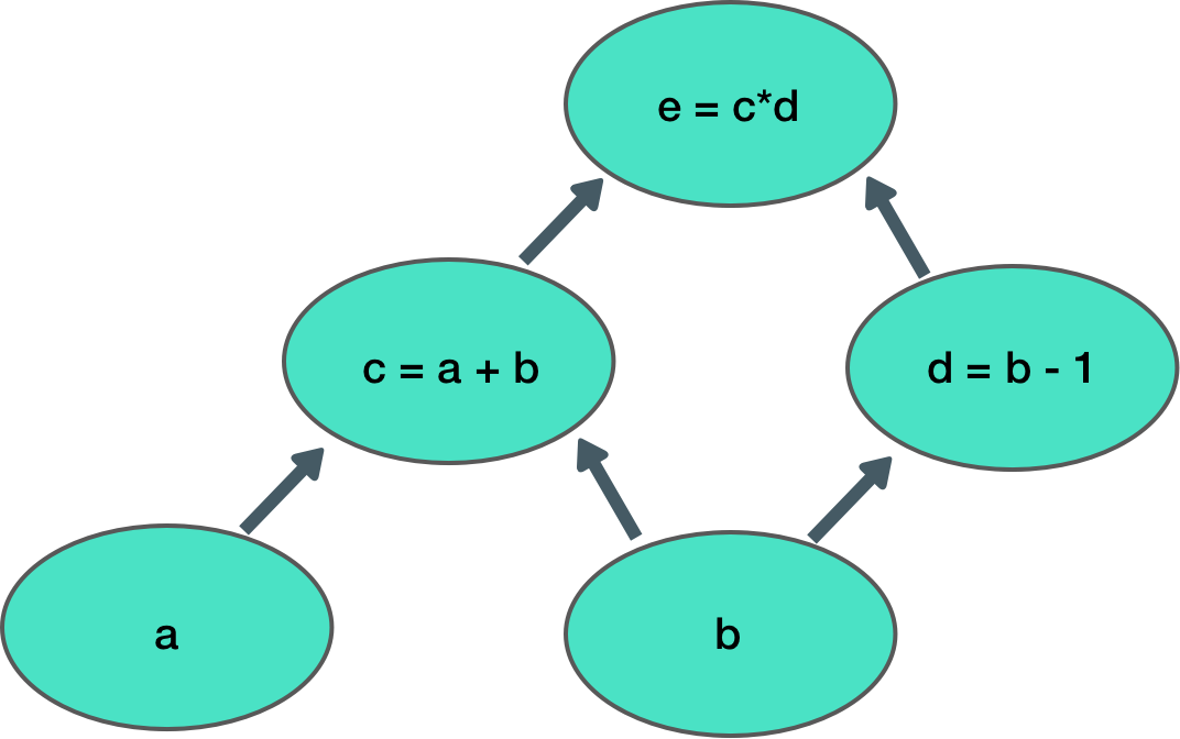
This graph takes 2 inputs, (a, b) and computes an output (e). Each node in the graph is an operation that takes some input, does some computation, and passes its output to another node.
We could make this computation graph in TensorFlow in the following way:
a = tf.placeholder(tf.float32)
b = tf.placeholder(tf.float32)
c = tf.add(a, b)
d = tf.sub(b, 1)
e = tf.mul(c, d)
Tensorflow uses tf.placeholder to handle inputs to the model. This is like making a reservation at a restaurant. The restaurant reserves a spot for 5 people, but you are free to fill those seats with any set of friends you want to. tf.placeholder lets you specify that some input will be coming in, of some shape and some type. Only when you run the computation graph do you actually provide the values of this input data. You would run this simple computation graph like this:
with tf.Session() as session:
    a_data, b_data = 3.0, 6.0
    feed_dict = {a: a_data, b:b_data}
    output = session.run([e], feed_dict=feed_dict)
    print(output) # 45.0
We use feed_dict to pass in the actual input data into the graph. We use session.run to get the output from the c operation in the graph. Since e is at the end of the graph, this ends up running the entire graph and returning the number 45 - cool!
Note that the computation graph we have defined is fixed + static. It can’t really learn anything. We’re now going to make a computation graph that can do some learning (hint hint: a neural network).
Our task: Sentiment Analysis
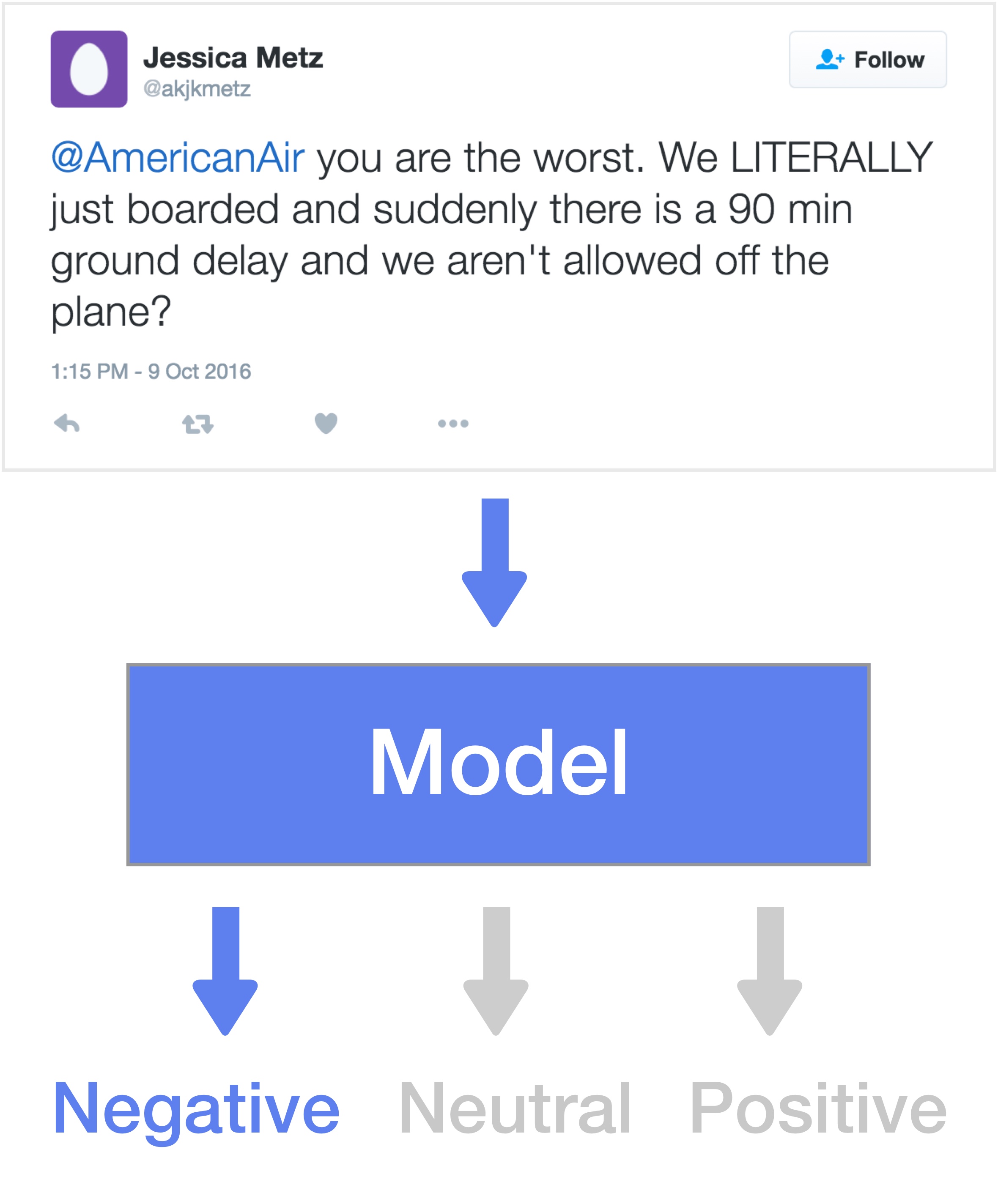
For this tutorial, we’re going to be learning a model to perform sentiment analysis on tweets. Given some tweet, we want our network to determine if the tweet is positive, negative, or neutral. This data can be downloaded here.
Building the Model
In this model, we’ll be representing tweets as bag-of-words (BOW) representations. BOW representations are vectors where each element index represents a different word and its value represents the number of times this word appears in our sentence. This means that each sentence will be represented by a vector that is vocab_size long. Our output labels will be represented as a vector of size n_classes (3). We get this data with some utility functions:
X, y, index_to_word, sentences = utils.load_sentiment_data_bow()
X_train, y_train, X_test, y_test = utils.split_data(X, y)
vocab_size = X.shape[1]
n_classes = y.shape[1]
So we have our data loaded as numpy arrays. But remember, TensorFlow graphs begin with generic placeholder inputs, not actual data. We feed the actual data in later once the full graph has been defined. We define our placeholders like this:
data_placeholder = tf.placeholder(tf.float32, shape=(None, vocab_size), name='data_placeholder')
labels_placeholder = tf.placeholder(tf.float32, shape=(None, n_classes), name='labels_placeholder')
A note about ‘None’ and fluid-sized dimensions:
You may notice that the first dimension of shape of data_placeholder is ‘None’. data_placeholder should have shape (num_tweets, vocab_size). However, we don’t know how many tweets we are going to be passing in at a time. Its possible that we only want to pass in 1 tweet at a time, or 30, or 1,000. Thankfully, TensorFlow allows us to specify placeholders with fluid-sized dimensions. We can use None to specify some fluid dimension of our shape. When our data eventually gets passed in as a numpy array, TensorFlow can figure out what the value of the fluid-size dimension should be.
Network Parameters
Let’s now define and initialize our network parameters:
# Define Network Parameters
n_hidden_units_h0 = 512
n_hidden_units_h1 = 256

h0_weights = tf.Variable(
    tf.truncated_normal([vocab_size, n_hidden_units_h0]),
    name='h0_weights')
h0_biases = tf.Variable(tf.zeros([n_hidden_units_h0]),
                     name='h0_biases')


h1_weights = tf.Variable(
    tf.truncated_normal([n_hidden_units_h0, n_hidden_units_h1]),
    name='h1_weights')
h1_biases = tf.Variable(tf.zeros([n_hidden_units_h1]),
                     name='h1_biases')

h2_weights = tf.Variable(
    tf.truncated_normal([n_hidden_units_h1, n_classes]),
    name='h2_weights')
h2_biases = tf.Variable(tf.zeros([n_classes]),
                     name='h2_biases')
We have defined our model parameters using tf.Variable. When you create a tf.Variable you pass a Tensor as its initial value to the Variable() constructor. A Tensor is a term for any N-dimensional matrix. There are a ton of different initial Tensor value functions you can use (full list). All these functions take a list argument that determines their shape. Here we use tf.truncated_normal for our weights, and tf.zeros for our biases. Its important that the shape of these parameters are compatible. We’ll be matrix-multiplying the weights, so the last dimension of the previous weight must equal the first dimension of the next weight. Notice this pattern in the Tensor initialization code. Lastly, notice the size of the Tensor for our last weights. We are predicting a vector of size n_classes so our network needs to end with n_classes nodes.
Computation Graph
Now let’s define our computation graph.
# Define Computation Graphs
hidden0 = tf.nn.relu(tf.matmul(data_placeholder, h0_weights) + h0_biases)
hidden1 = tf.nn.relu(tf.matmul(hidden0, h1_weights) + h1_biases)
logits = tf.matmul(hidden1, h2_weights) + h2_biases
Lets break this down. So our first operation in our graph is a tf.matmul of our data input and our first set of weights. tf.matmul performs a matrix multiplication of two tensors. This is why it is so important that the dimensions of data_placeholder and h0_weights align (dimension 1 of data_placeholder must equal dimension 0 of h0_weights). We then just add the h0_bias variable and perform a nonlinearity transformation (we use tf.relu for a rectified linear unit (relu). We do this again for the next hidden layer, and the final output logits.
Loss Functions
We have defined our network, but we need a way to train it. Training a network comes down to optimizing our network to minimize a loss function. Here we define our loss function and optimization strategy.
# Define Loss Function + Optimizer
loss = tf.reduce_mean(
    tf.nn.softmax_cross_entropy_with_logits(logits, labels_placeholder))
learning_rate = 0.0002
optimizer = tf.train.GradientDescentOptimizer(learning_rate).minimize(loss)
prediction = tf.nn.softmax(logits)
prediction_is_correct = tf.equal(
    tf.argmax(logits, 1), tf.argmax(labels_placeholder, 1))
accuracy = tf.reduce_mean(tf.cast(prediction_is_correct, tf.float32))
This is a classification problem, so our loss for each example is just the cross entropy of our prediction and the label. We train this one minibatch at a time, so we average the loss of all the examples in our minibatch to get the minibatch loss which we use to update the network parameters. We use Gradient Descent via tf.train.GradientDescentOptimizer and minimize this loss. We also define a way to compute accuracy for later logging of results.
Quick Conceptual Note:
Nearly everything we do in TensorFlow is an operation with inputs and outputs. Our loss variable is an operation, that takes the output of the last layer of the net, which takes the output of the 2nd-to-last layer of the net, and so on. Our loss can be traced back to the input as a single function. This is our full computation graph. We pass this to our optimizer which is able to compute the gradient for this computation graph and adjust all the weights in it to minimize the loss.
Training our Net
We have our network, our loss function, and our optimizer ready, now we just need to pass in the data to train it. We pass in the data in chunks called mini-batches.
# Train loop

num_steps = 1000
batch_size = 128

tf.initialize_all_variables().run()

for step in xrange(num_steps):
    offset = (step * batch_size) % (X_train.shape[0] - batch_size)
    # Generate a minibatch.
    batch_data = X_train[offset:(offset + batch_size), :]
    batch_labels = y_train[offset:(offset + batch_size), :]
    feed_dict_train = {data_placeholder: batch_data, labels_placeholder : batch_labels}
    # Run the optimizer, get the loss, get the predictions.
    # We can run multiple things at once and get their outputs
    _, loss_value_train, predictions_value_train, accuracy_value_train = session.run(
      [optimizer, loss, prediction, accuracy], feed_dict=feed_dict_train)
    if (step % 10 == 0):
        print "Minibatch train loss at step", step, ":", loss_value_train
        print "Minibatch train accuracy: %.3f%%" % accuracy_value_train
        feed_dict_test = {data_placeholder: X_test, labels_placeholder: y_test}
        loss_value_test, predictions_value_test, accuracy_value_test = session.run(
            [loss, prediction, accuracy], feed_dict=feed_dict_test)
        print "Test loss: %.3f" % loss_value_test
        print "Test accuracy: %.3f%%" % accuracy_value_test
Running this code, you’ll see the network train and output its performance as it learns. I was able to get it to 65.5% accuracy. This is not great considering random guessing gets you 33.3% accuracy. We’ll cover numerous ways to improve upon this in later tutorials.
Concluding Thoughts
This was a brief introduction into TensorFlow. There is so, so much more to learn and explore, but hopefully this has given you some base knowledge to expand upon. As an exercise: see what you can do with this code to improve the performance. Ideas include: randomizing mini-batches, making the network deeper, using RNN’s on word tokens instead of fully connected layers on bag-of-words, trying different optimizers (like Adam), different weight initializations. We’ll explore some of these in future tutorials.
Note:
All of code from this post can be found here. The original Google Slides presentation can be found here.
HackerNews discussion: here.
Questions? Reach out to nicholasjlocascio at gmail dot com